May 17, 2016

KS Curve plot

Today I’ll present a simple R function to create a plot for the metric KS. I’m assuming that you are familiar with this metric and your usage.

As I told in the previous post ROC Curve plot and AUC I always recommend to also check the plot of some metrics, instead of only being satisfied by the value of the metric. This will help you to make sure that your model’s predictions are ok along the whole range of probabilities.

Again, remember that we are considering the scenario of a binary classifier.

The R function I wrote to evaluate the KS Curve can be found here. Unlike the ROC Curve function, this one cannot be used to do comparisons among groups in the same plot. I recommend you to create a plot for each one of the groups. In the following example, we’ll do that for the train and a valid subsets of data.

# Goodness of Fit Metrics 'KS plot' (for prediction models with target [0;1])

funcGFMplotKS = 
function (var.target="", var.prediction="", var.df="", var.fsize)
{
    ...
}

So let’s get practical and see how it works!

This is an example of a function call. In this case, all the records in the tmp_train data frame is regarding the train subset.

> unique(tmp_train$Scenario)
[1] "Train"

The var.fsize parameter is the reference for the text font size used in ggplot2. Default value is set to 3.

funcGFMplotKS (var.target="target", var.prediction="pred", var.df="tmp_train", var.fsize=3)

This is the result:

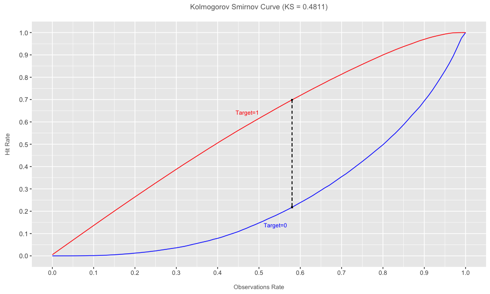
The black dashed line (- - -) identifies the exact point where the curves reach the maximum distance from each other. This is the known KS value. If you’re curious about how the calculation is done you can check it directly in the R code available here.

Now, this is the result if we call the same function to the valid data frame:

> unique(tmp_valid$Scenario)
[1] "Valid"
funcGFMplotKS (var.target="target", var.prediction="pred", var.df="tmp_valid", var.fsize=3)

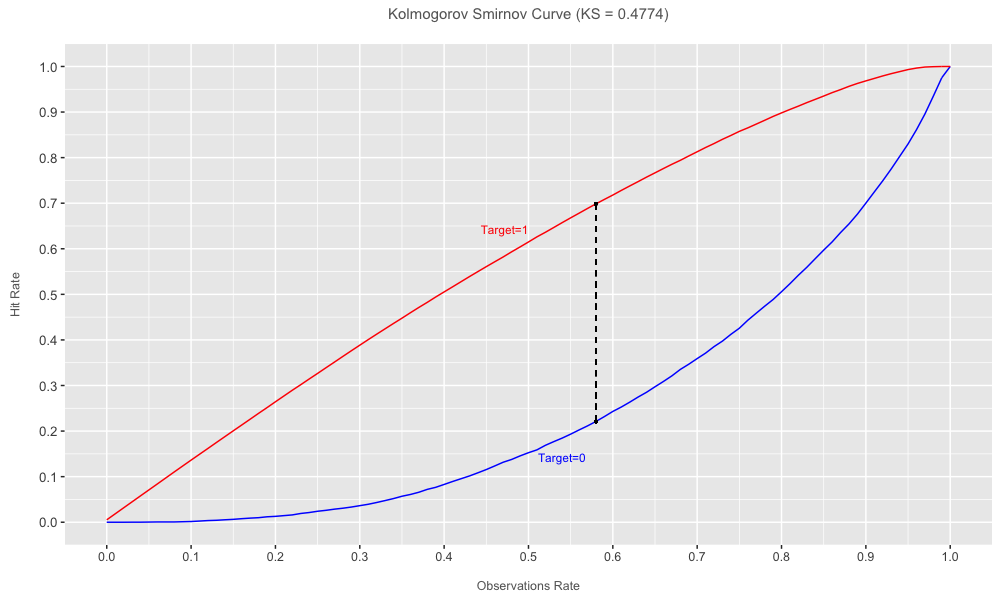
Note that the chart title shows different values of the KS. And these values match exactly the same values calculated by the funcGFMmetrics function, presented in an earlier posting.

# TRAIN data frame
metrics = funcGFMmetrics (var.target="target", var.prediction="pred", var.df="tmp_train")    
> metrics
    AUC        KS      GINI   LogLoss     Kappa        F1  Accuracy ErrorRate Precision    Recall 
0.82913   0.48114   0.65826   0.77364   0.40113   0.81346   0.74074   0.25926   0.89988   0.74219


# VALID data frame
metrics = funcGFMmetrics (var.target="target", var.prediction="pred", var.df="tmp_valid")    
> metrics
    AUC        KS      GINI   LogLoss     Kappa        F1  Accuracy ErrorRate Precision    Recall 
0.82547   0.47744   0.65095   0.76664   0.39905   0.81350   0.74053   0.25947   0.89661   0.74450

This can be quite handy ¹, specially if you usually write (and automate) reports documenting your development and evaluation model processes, or even if you have some R code procedures running periodically to follow up the model performance that are delivered to your clients.

That’s all folks! ;-)

To make sure all your outputs are exactly the same. ↩

KS Curve plot

Related Posts